Getting started with ggmeta

ggmeta turns a meta-analysis into a publication-quality forest plot built on ggplot2. It works two ways:

on a meta object (from the meta package), or
on a plain tidy data frame — no meta package required.

Because the result is an ordinary ggplot, you keep the full ggplot2 toolbox: themes, scales, annotations, and saving with ggsave().

library(ggmeta)
library(ggplot2)

A forest plot from a `meta` object

Fit a meta-analysis as usual, then hand it to ggforest():

library(meta)
#> Loading required package: metabook
#> Loading 'meta' package (version 8.5-0).
#> Type 'help(meta)' for a brief overview.

m <- metabin(
  event.e = c(14, 30, 15, 22), n.e = c(100, 150, 100, 120),
  event.c = c(10, 25, 12, 18), n.c = c(100, 150, 100, 120),
  studlab = c("Study A", "Study B", "Study C", "Study D"),
  sm = "RR"
)

ggforest(m)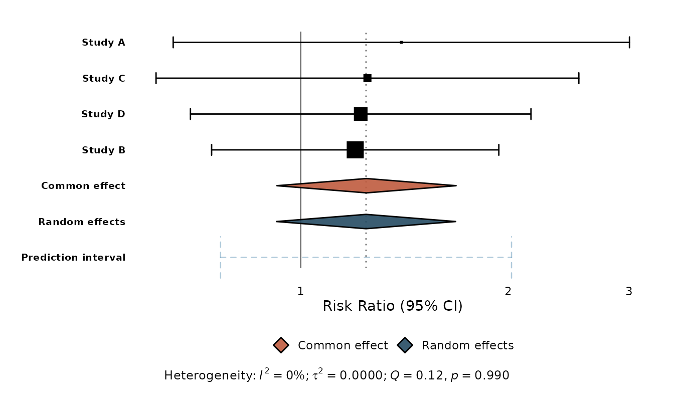

ggforest() does the sensible thing automatically: it draws study confidence intervals with weight-proportional squares, the common- and random-effects summary diamonds, a prediction interval, a null-effect reference line, a log x-axis for ratio measures, and a heterogeneity caption.

Standalone: a tidy data frame

You don’t need the meta package. Any data frame with studlab, estimate, ci_lower, and ci_upper works:

df <- data.frame(
  studlab  = c("Trial 1", "Trial 2", "Trial 3", "Trial 4"),
  estimate = c(0.82, 0.91, 0.68, 1.05),
  ci_lower = c(0.61, 0.74, 0.48, 0.80),
  ci_upper = c(1.10, 1.12, 0.96, 1.38)
)

ggforest(df, null_effect = 1)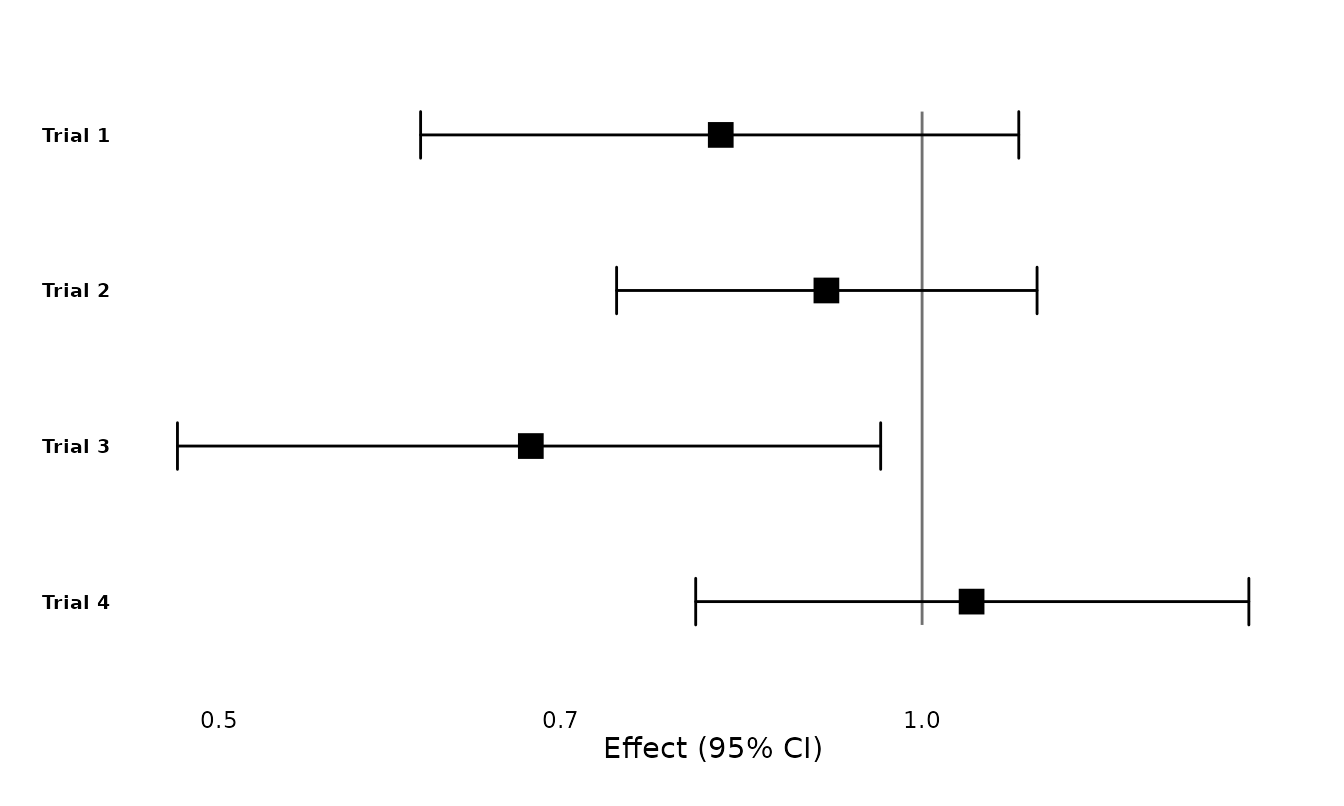

On-the-fly meta-analysis

Give ggforest() a se column (or let it recover the standard error from the confidence interval) and set add_summary = TRUE to pool the studies with an inverse-variance common-effect and a DerSimonian–Laird random-effects model — without the meta package:

studies <- data.frame(
  studlab  = c("Trial 1", "Trial 2", "Trial 3", "Trial 4", "Trial 5"),
  estimate = c(0.10, 0.35, 0.22, 0.48, 0.05),
  se       = c(0.12, 0.10, 0.14, 0.16, 0.11)
)
studies$ci_lower <- studies$estimate - 1.96 * studies$se
studies$ci_upper <- studies$estimate + 1.96 * studies$se

ggforest(studies, add_summary = TRUE)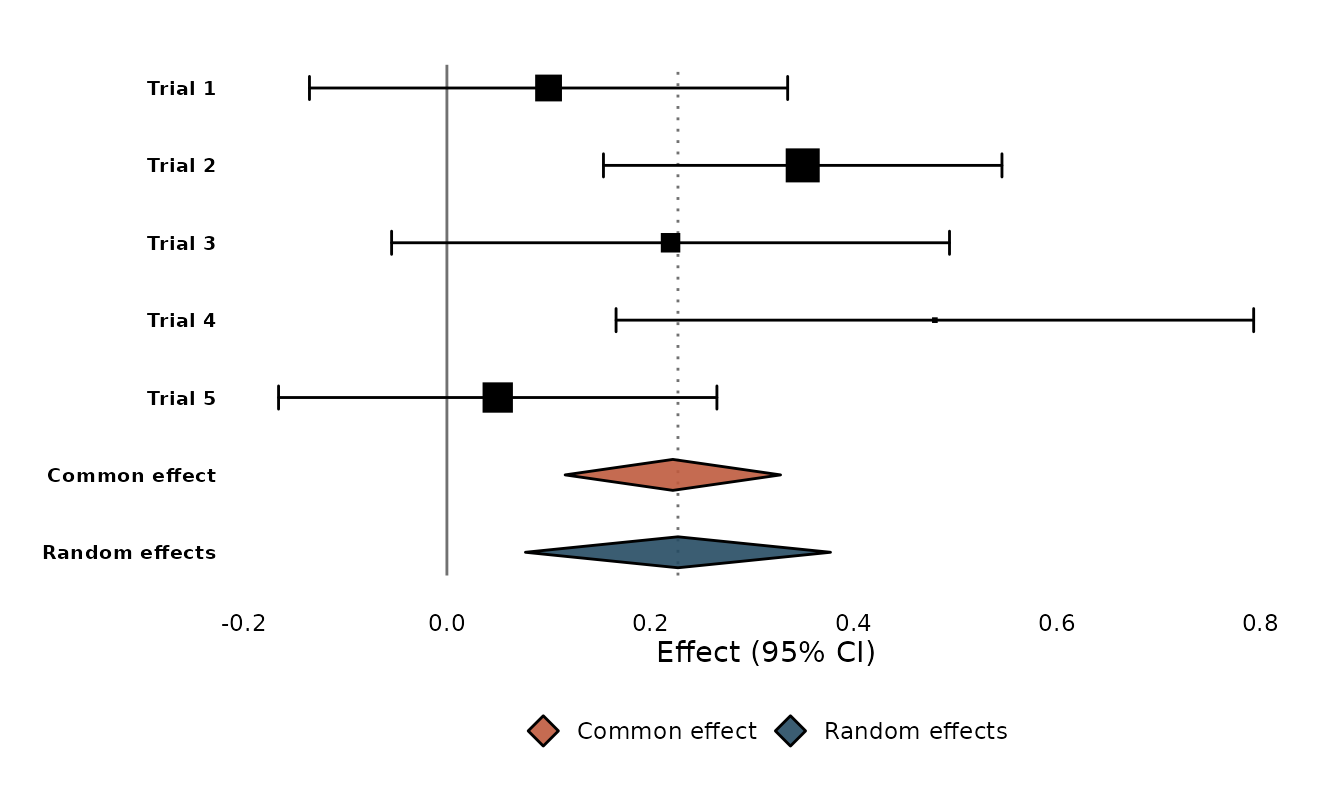

A `meta::forest()`-style column table

Set columns = TRUE to add the familiar effect / 95% CI / weight columns with headers to the right of the plot (use effect_header to name the estimate column, and pass a subset like columns = c("estimate", "ci") if you prefer):

ggforest(studies, add_summary = TRUE, columns = TRUE, effect_header = "SMD")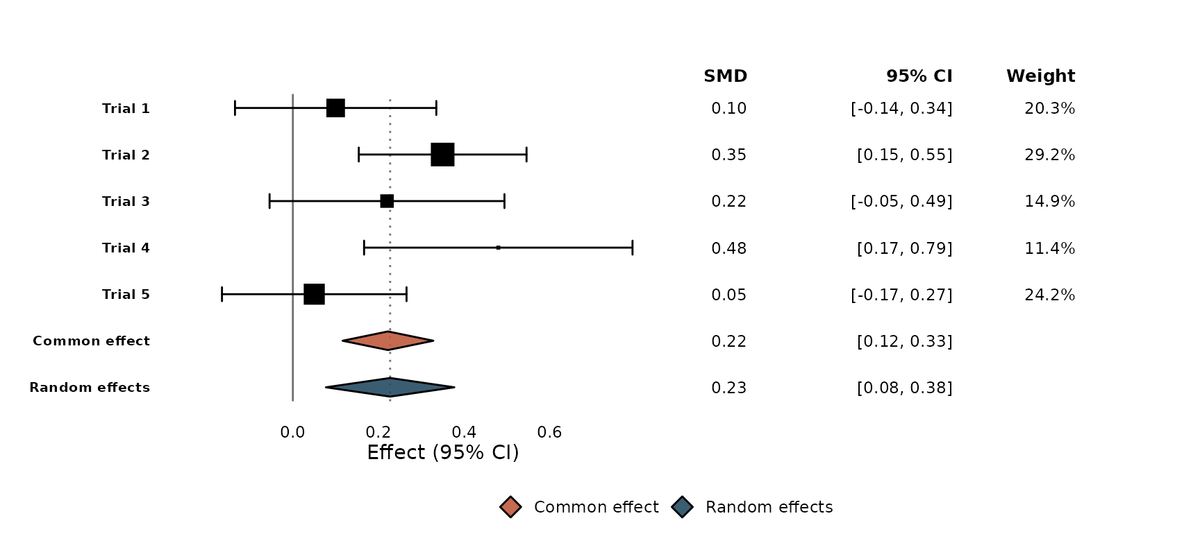

Custom text columns

For a column of your own — sample sizes, events, anything — use geom_forest_text(), which aligns to the study rows through the shared y. format_effect() builds an “estimate (CI)” label. Widen the panel with expand_limits() to make room:

studies$n <- c(120, 240, 150, 180, 110)

ggforest(studies, add_summary = TRUE) +
  geom_forest_text(aes(y = studlab, label = n), data = studies,
                   x = -0.35, hjust = 0.5) +
  expand_limits(x = -0.45)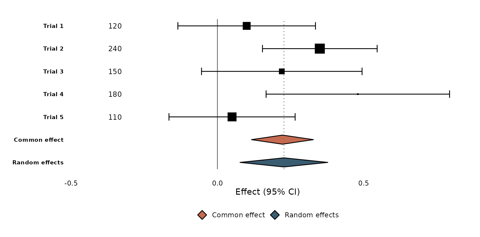

Journal styles

Layout presets adapt a plot to common journal conventions. They are ordinary ggplot2 components, so you add them with +:

p <- ggforest(df, null_effect = 1)
layout_jama(p)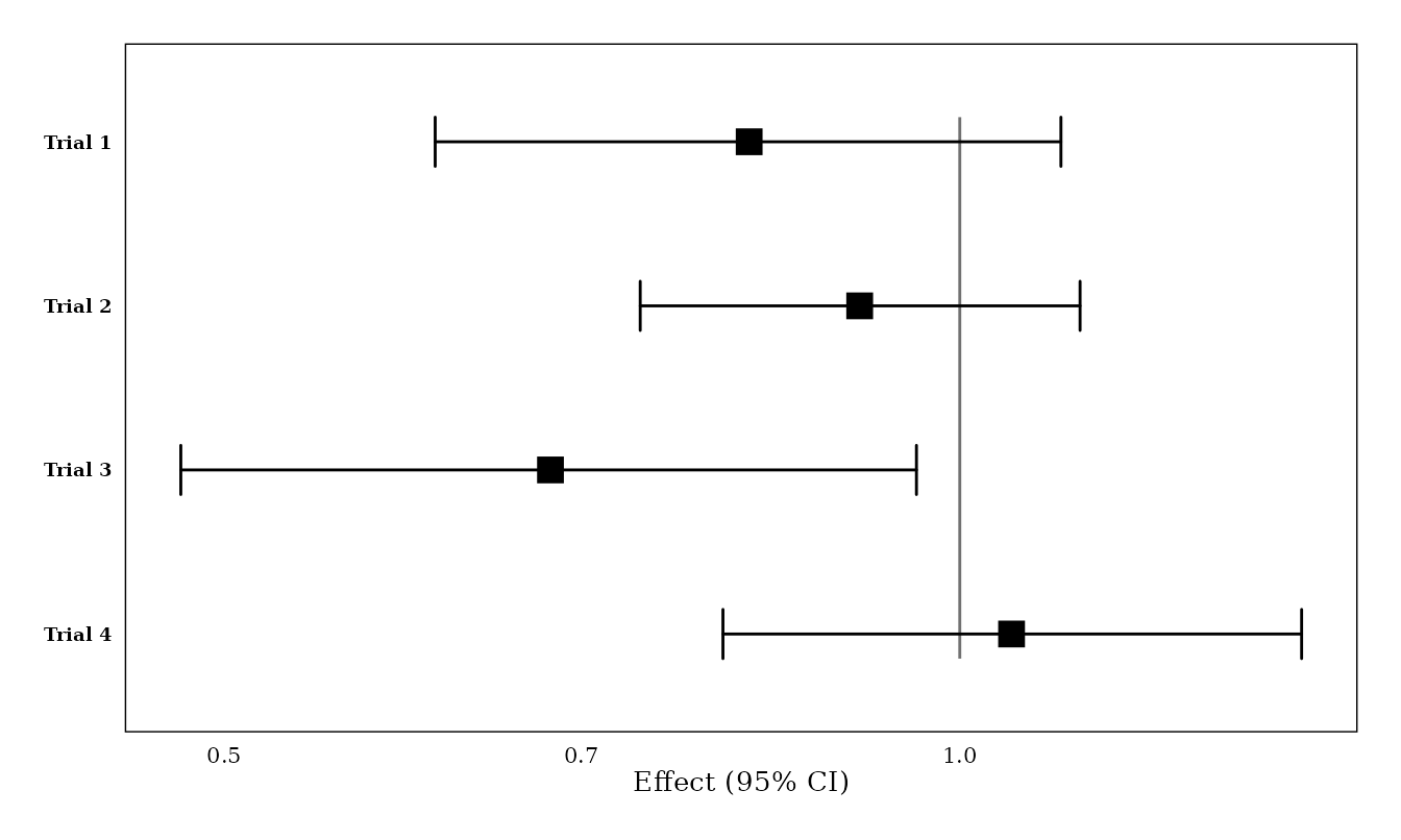

layout_bmj() and layout_revman5() are also available, and because the plot is a ggplot you can keep customising with theme(), labs(), and friends.

Other effect measures

ggforest() back-transforms every summary measure correctly — exponentiation for ratios, inverse-logit for logit proportions, Fisher’s z for correlations, and so on. Single-group proportions and rates get no (meaningless) reference line:

prop <- metaprop(
  event = c(15, 20, 12, 25), n = c(50, 60, 55, 70),
  studlab = paste("Cohort", 1:4), sm = "PLOGIT"
)
ggforest(prop)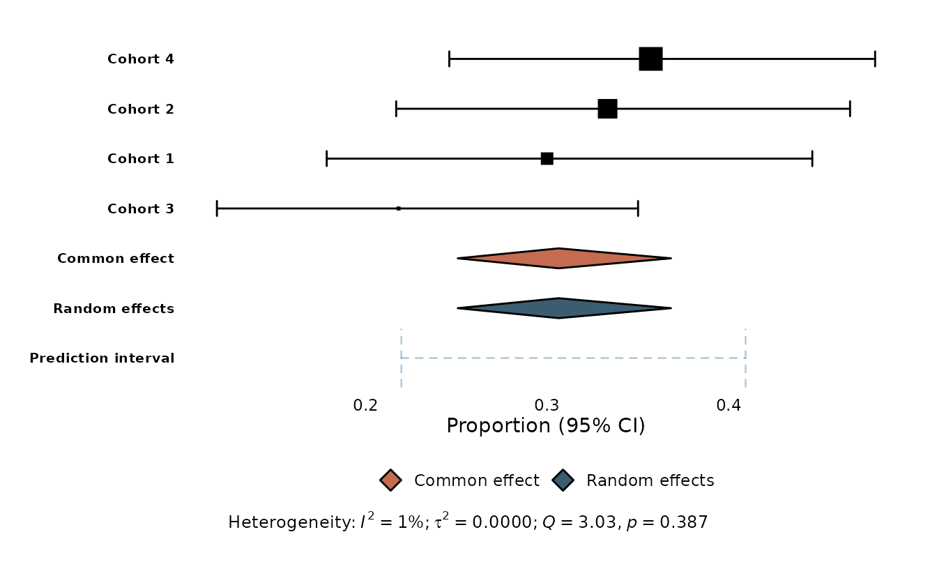

Saving

ggforest() returns a ggplot, so save it like any other:

p <- ggforest(df, null_effect = 1)
ggsave("forest.png", p, width = 7, height = 4, dpi = 300)

Where to next

See vignette("from-meta-forest") for a side-by-side comparison with meta::forest() and tips on reproducing its output.

A forest plot from a meta object