Study-level confidence intervals and point estimates for forest plots
Source:R/geom-forest-ci.R
geom_forest_ci.Rdgeom_forest_ci() draws a confidence interval line and a
weight-proportional square for each study in a forest plot.
The square area scales with the study weight, making more precise
studies visually prominent.
Usage
geom_forest_ci(
  mapping = NULL,
  data = NULL,
  stat = "forest_ci",
  position = "identity",
  ...,
  ci_width = 0.3,
  point_size_range = c(1, 6),
  na.rm = FALSE,
  show.legend = NA,
  inherit.aes = TRUE
)
Arguments
- mapping
Set of aesthetic mappings created by
aes(). If specified andinherit.aes = TRUE(the default), it is combined with the default mapping at the top level of the plot. You must supplymappingif there is no plot mapping.- data
The data to be displayed in this layer. There are three options:
If
NULL, the default, the data is inherited from the plot data as specified in the call toggplot().A
data.frame, or other object, will override the plot data. All objects will be fortified to produce a data frame. Seefortify()for which variables will be created.A
functionwill be called with a single argument, the plot data. The return value must be adata.frame, and will be used as the layer data. Afunctioncan be created from aformula(e.g.~ head(.x, 10)).- stat
The statistical transformation to use on the data for this layer. When using a
geom_*()function to construct a layer, thestatargument can be used to override the default coupling between geoms and stats. Thestatargument accepts the following:A
Statggproto subclass, for exampleStatCount.A string naming the stat. To give the stat as a string, strip the function name of the
stat_prefix. For example, to usestat_count(), give the stat as"count".For more information and other ways to specify the stat, see the layer stat documentation.
- position
A position adjustment to use on the data for this layer. This can be used in various ways, including to prevent overplotting and improving the display. The
positionargument accepts the following:The result of calling a position function, such as
position_jitter(). This method allows for passing extra arguments to the position.A string naming the position adjustment. To give the position as a string, strip the function name of the
position_prefix. For example, to useposition_jitter(), give the position as"jitter".For more information and other ways to specify the position, see the layer position documentation.
- ...
Other arguments passed on to
ggplot2::layer(). These are often aesthetics, used to set an aesthetic to a fixed value, likecolour = "red"orlinewidth = 1.- ci_width
Width of the CI line end-marks as a proportion of the spacing between study rows. Default:
0.3.- point_size_range
Minimum and maximum point size in mm. Default:
c(1, 6). The side of each square ismin + (max - min) * sqrt(weight / max(weight)), i.e. the part above the minimum grows with the square root of the weight. Missing or non-positive weights get the minimum size; when no study has a usable weight there is nothing to scale, so every square is drawn at the middle of the range (asmeta::forest()does for amethod = "GLMM"fit). A constantsize(or a mappedsizeaesthetic) overrides the weight-based size.- na.rm
If
FALSE(default), missing values are removed with a warning. IfTRUE, missing values are silently removed.- show.legend
logical. Should this layer be included in the legends?
NA, the default, includes if any aesthetics are mapped.FALSEnever includes, andTRUEalways includes. It can also be a named logical vector to finely select the aesthetics to display. To include legend keys for all levels, even when no data exists, useTRUE. IfNA, all levels are shown in legend, but unobserved levels are omitted.- inherit.aes
If
FALSE, overrides the default aesthetics, rather than combining with them. This is most useful for helper functions that define both data and aesthetics and shouldn't inherit behaviour from the default plot specification, e.g.annotation_borders().
Aesthetics
geom_forest_ci() understands the following aesthetics
(required aesthetics are in bold):
x— point estimatexmin— lower confidence limitxmax— upper confidence limity— study position (usually a factor)weight— study weight for square sizingcolour— line and square border colour (default: "black")fill— square fill colour (default: "black")alpha— transparency (default: 1)linewidth— CI line width (default: 0.5)size— override for square size; computed from weight by defaultlinetype— CI line type (default: "solid")
Examples
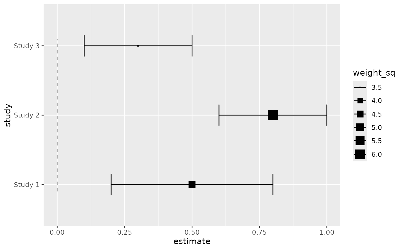
library(ggplot2)
df <- data.frame(
  study = c("Study 1", "Study 2", "Study 3"),
  estimate = c(0.5, 0.8, 0.3),
  lower = c(0.2, 0.6, 0.1),
  upper = c(0.8, 1.0, 0.5),
  weight = c(1, 2, 0.5)
)
ggplot(df, aes(y = study, x = estimate, xmin = lower, xmax = upper,
               weight = weight)) +
  geom_forest_ref() +
  geom_forest_ci()